
State of Charge Estimation with a Kalman Filter
Last Updated: 5/13/19
State of charge (SoC) estimation is vitally important for practical battery applications. Here, I use a Kalman Filter running on Python and Arduino to estimate the SoC of the batteries.
State of Charge Estimation
Since a battery’s state of charge (SoC) cannot be directly measured, it is estimated using state variables of related characteristics—namely the battery’s open circuit voltage (OCV) and the current leaving or entering the cell; however, neither of these methods are sufficient on their own. The cell's OCV measurement is noisy and cannot be constantly measured as it requires disconnecting whatever device the battery is powering. Additionally, estimating the SoC by coulomb counting (measuring every charge leaving or entering the cell) gradually produces significant error over long time intervals. By dynamically combining these two measurements, though, a more accurate estimate can be achieved. Enter, the Kalman Filter.
Index
Kalman Filter Example: A Car on a Road Trip in the Dark
The Situation: Let’s say we’re going on a road trip and there’s a very important turn we can’t afford to miss at mile marker N. Unfortunately, it's pitch black and we can’t see the turn unless we’re exactly there or we already passed it; however, past the turn is a town of outlaws, so it’s quite dangerous to miss the turn.

What We Know: We left our hometown at time T_initial from position X_initial. In our car, we have a speedometer with a stopwatch, along with a GPS device that is only accurate to 100 feet and can only measure position every 3 minutes.
The Question: How do we accurately measure our position so we don’t miss the turn?
Speedometer Method: We take periodic time measurements with our stop watch, then multiply the time interval by the speed on the speedometer to calculate distance traveled. We then add that distance to our initial position and repeat the process over and over until we think we are at mile N.
Issue: Over time, small errors from tire slippage, wind blowing the car, small deviations from perfectly straight steering, and noise from our speedometer will build up to produce an inaccurate measurement.

GPS Method: We take a GPS reading every 3 minutes and hope that we happen to take our measurement when we pass the turn (and that there is no noise in the reading)
Issue: We have long periods where we don’t know our position, and even when do get a measurement it is noisy and only accurate to 100 feet. Chances are we miss miss the turn.

The Solution: Dynamically combine the two methods with sensor fusion in a Kalman Filter
“Cross check” our estimates at each GPS reading, then re-start our estimate from that point

How a Kalman Filter Works

Visualization of multiplying two Gaussians together, from https://www.bzarg.com/p/how-a-kalman-filter-works-in-pictures/
Underlying Math
The Kalman Filter assumes that all states and measurements can be represented as normal Gaussian distributions with a mean and covariance. Think of the pink Gaussian as GPS and the green Gaussian as our speedometer estimate. When we combine our two estimates (multiply the Gaussians), we get a Gaussian with a new mean and smaller variance, i.e. a more accurate estimate (the blue Gaussian)

Estimation Iterations (Simplified):
The Kalman Filter operates in 3 key phases:
Predict: the system’s state is estimated using some model that describes the system’s dynamics (like multiplying the car’s speed by a known time interval to guess the distance traveled)
Measure: an actual measurement of the system is taken (like taking a GPS reading)
Update: the Kalman Filter dynamically weights the state prediction and noisy state measurement to give us a more precise estimate of the true system state
That updated state estimate is then used as the starting point for the next prediction, and the Kalman Filter recursively estimates the current state based on the last estimate. Because of this recursive behavior, a Kalman Filter uses small amounts of memory as it does need the entire record of previous states to estimate the next one.
The Battery Model
Going off of the road trip example, the “position” we want to estimate is the state of charge of the battery. For the battery system, we use measurements of the current into or out of the cell and open circuit voltage of the cell.
Current measurement = speedometer
We can constantly measure the current leaving or entering the battery, then multiply the measured current by a time interval to get the total number of coulombs that have left the cell
Open circuit voltage measurement = GPS
While the open circuit voltage gives us a very good idea of the battery’s state of charge, we can’t frequently measure it as it requires disconnecting the power supply to whatever device the battery is powering
Relating State of Charge to Open Circuit Voltage
Data Collection
To get a function that computes the state of charge of the cell based on its open circuit voltage, I first had to collect data on the cell’s open circuit voltage as it went from 100% to 0% charge. Since a true open circuit voltage discharge would take months waiting for the battery’s self discharge to drain the cell, I used a quasi-OCV discharge where the battery drained at C/20 (the cell’s capacity / 20). Since I am using Samsung 18650 cells with a 3Ah capacity, this corresponds to a discharge rate of 150mA. Using Ohm’s Law, I needed a resistor of R = V/I = 3.7V/.15A = 25 Ohms. The closest power resistor I had was 30 Ohms, so I put the 30 Ohm resistor in series with one 18650 cell and measured the voltage drop across the cell using an Arduino from 4.1V to 2.5V.

The Open Circuit Voltage Measurement Circuit Schematic
An Arduino measures the voltage drop across the cells using an analog pin.

A Picture of the Open Circuit Voltage Measurement Circuit
The Arduino is connected via USB to my MacBook, which runs a Python script that reads the OCV values from the Arduino and writes them to a .csv file
The Arduino writes the OCV measurement to the Serial monitor, from which a Python script reads the value and writes it to a .csv file for data analysis. During data collection, the Arduino collected over 50k data points during a ~21 hour discharge.
The Arduino code can be found here: Arduino_voltmeter_final.ino
The Python code can be found here: Arduino_serial_reader.py
The raw battery data can be found here: Raw Battery Data.csv
The Python code used for data analysis can be found here: Battery Data Analysis.py
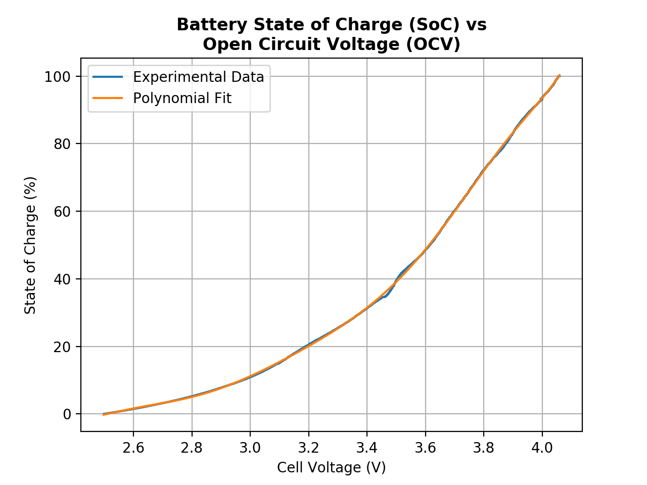
An 8th Order Polynomial Fit of the Battery Quasi-OCV Discharge
The polynomial fit allows me to get a SoC estimate for a given OCV measurement
Data Analysis
I first took measurements as [measurement number, OCV], then normalized the data points to a 0 to 100% scale, from which I fit a polynomial function to get the state of charge as a function of open circuit voltage. The Python script I wrote conducted a minimum chi square analysis to determine the optimal order fit and arrived at an 8th order function. The average chi square value for the 8th order fit was an order of magnitude less than the 2nd through 7th order fits.
This gave me to state of charge (SoC) as a function of open circuit voltage (OCV). The coefficients of the 8th order polynomial fit are:

A matrix view of the SoC(OCV) function
SoC(OCV) =
268.4970355259198 * OCV^8 +
-6879.270367122276 * OCV^7 +
76716.49575172913 * OCV^6
-486365.6733759814 * OCV^5
1917287.1707991716 * OCV^4
-4812471.06572991 * OCV^3
7511312.300797121 * OCV^2
-6665390.783393391 * OCV
2574719.229612701
Relating State of Charge to Current

The Current Measurement Circuit Schematic
An Arduino measures the voltage drop across R-Ammeter, then uses Ohm’s Law to calculate a current and sends it to Python via Serial.
Data Collection
Using a similar circuit to the Arduino voltmeter, I put the Li-ion cell in series with a 1Ω power resistor and a 60Ω test load. The Arduino measures the voltage drop across the power resistor, then using Ohm’s Law: I=V/R, where R is precisely measured to be R = 1.036 +/- 0.011Ω. the Arduino then sends this current value to Python via the Serial monitor.
Using Current to Find Lost/Gained Charge
The 18650 cell is rated at 3Ah, so we can easily calculate the total number coulombs the battery can hold. We can then calculate the coulombs used from our current reading. By dividing the coulombs used over our total coulombs, we get the state of charge used. And by subtracting/adding that to the initial state of charge, we end up with the state of charge as a function of time and current.


System Overview (Software & Hardware)

System Diagram
Python controls the Arduino via the serial monitor, and Arduino manipulates which mode of data collection the circuit is in.
With the state of charge of the battery as a function of open circuit voltage, I could move on to developing the actual circuit and hardware used to operate the Kalman Filter. The circuit needs to be able to measure the current leaving or entering the batteries, but also have some mechanism to disconnect the cells from load to measure their open circuit voltage.

Picture of the System in Operation
All systems are labeled according to the diagram above.
Python is the brain behind this system’s operation. It controls the circuit via commands that it sends to Arduino, which then controls which mode of data collection the circuit is in. Two Li-ion cells are connected directly to the circuit, and they discharge through it to load.
Kalman Filter Circuit
I developed the below circuit to combine current and open circuit voltage measurement on one device, which a single Arduino controls. It operates in two states:
Current Measurement: When the relay is off, the battery is connected to load and discharges through the ~1Ω power resistor. The Arduino measures the voltage drop across R-Power to determine the current and sends this value to Python.
OCV Measurement: When the relay is on via a HIGH digital write from Arduino, the battery is disconnected from load so that an OCV measurement can be taken. The Arduino measures the voltage drop across R1 (which creates a voltage divider with R2) and sends this value to Python.

Relay Off: Current Measurement
The battery is connected to load and discharges through R-Power. Arduino measures the voltage drop across R-Power by measuring the drop between A0 and GND.

Relay On: OCV Measurement
Arduino writer D2 to HIGH, which energizes the relay and disconnects the batteries from load. Arduino measures the voltage drop between A1 and GND to determine the OCV of the batteries. R1 and R2 create a voltage divider so the OCV reading stays within the Arduino’s 5V measurement bounds.
Kalman Filter Algorithm
To demonstrate how the Kalman Filter algorithm works, we’ll go through a sample iteration: initialization, prediction, measurement, update (where the Kalman Filter does its thing).
**Throughout the demonstration, two indices (t and t-1) are used to denote states. The “t” index represents the current state, and the “t-1” index represents the last state.
Initialization
Python tells Arduino to measure OCV and current, which are used to initialize the state estimate matrix. The estimate variance matrix is also initialized. In my case, I used values of ~0.5, knowing that these are supposed to be higher than the observation variance matrix to allow the Kalman Filter to properly “train” itself. I found that essentially regardless of what the initial estimate variance is, the estimate tends to be the same over long periods of time (shown in the Test Data section).

Predict: Periodic Current Measurements
For each prediction iteration, the transformation matrix is updated with the time interval over which current was measured. (This is like measuring the car’s speed with the speedometer and multiplying it by time).

We then multiply the state transformation matrix by the last state to get the new state estimate and variance. We also take a new current measurement with the Arduino to update second component of the state estimate matrix.

Conceptually, we’re essentially using this equation (same form as position = initial position + velocity*time)

Measure: Take an OCV Measurement
We first initialize the observation matrix, which in this case is the identity matrix since we are using raw sensor data without manipulation.

We then measure the OCV to get the state measurement.

We also initialize the observation noise matrix. I set this value much lower than my estimation variance matrix to indicate to the Kalman Filter that I “trust” the OCV-determined state of charge more than my coulomb-counting-determined state of charge.

Update: Calculate Kalman Gain
We first calculate the residual vector (the difference between our measured and estimated state).

We then calculate the residual variance matrix.

Finally, we calculate the Kalman gain, which essentially tells us how much to weight our estimate vs our observation.

Update: Adjust the State Estimate with Kalman Gain
To get our new best estimate, we add the residual vector multiplied by the Kalman gain to the state estimate.

Additionally, we update the estimate variance matrix using the Kalman gain.

Repeat: Set the New Estimate as the Last Estimate
This is where the beauty of the Kalman Filter’s iterative nature comes in. We use the new best estimate as the starting point for our next iteration of state predictions. Thus, in terms of memory, we only need to keep track of our system model, the last state, and the current state. We don’t need the entire historical record of charge and discharge data to make our estimate.
So, we set the new state estimate as the last state estimate and set the new estimate variance matrix as the last estimate variance matrix.


And that’s it for the Kalman Filter algorithm! It recursively estimates the state of charge of the battery by combining current and OCV measurement data based on some underlying system model (coulomb counting).
The Python code used to run the above system and Kalman Filter can be found here: kalman_filter_operation.py
Test Data
In testing my Kalman Filter, I wanted to determine two things: Is the Kalman Filter’s estimate better than…
purely using current and time (coulomb counting) {speedometer method}?
purely using periodic OCV measurements {GPS method}?
I also wanted to see how accurate the Kalman Filter would be over long estimation periods. To answer these questions, I began by running a 7 hour discharge of the cells and tracked the coulomb counting estimate, the OCV estimate, the Kalman Filter estimate, and the “true” state of charge (a linear connection of OCV measurements).
Experimental Test: 7 Hour Discharge
I used the following experimental variance matrices to run the Kalman Filter. I figured my OCV -> SOC measurement would be accurate to about 0.5%, so the variance would be my uncertainty squared (.5*.5=.25). I then set the estimate variance as some value twice as large as my measurement variance. (P is the estimate, R is the observation)

Experiment results:

Kalman Filter vs Other Methods - State of Charge Estimate
The Kalman Filter is more accurate than coulomb counting and beats pure OCV measurements for about half of the experiment.

Kalman Filter vs Other Methods - Difference from “True” State of Charge
The Kalman Filter’s estimate is nearly twice as accurate as pure coulomb counting.
As the data above shows, the Kalman Filter (green) was undoubtedly more accurate than coulomb counting (blue). The Kalman Filter estimate gradually diverged from the OCV prediction, but beat it for nearly half of the estimation period. By the end of the estimation period, the Kalman Filter only differed from the true state of charge by 3%. This was nearly half of the coulomb counting’s 5.5% divergence.
Acknowledgement: In this experiment, the OCV was measured every 10 minutes. This would not be possible in a real implementation since the device the batteries are powering would need to be turned off every 10 minutes. The frequent OCV measurements allowed me to understand the behavior of my Kalman Filter better by increasing the number of iterations per measurement period. I am using these insights to improve the estimation between OCV measurements.
Adjustments Between Experiments: Improving Accuracy
In an attempt to improve the accuracy of the Kalman Filter, I did two things:
I increased the current measurement frequency from every 30s to every 10s. Perhaps current was changing more rapidly than I thought and my prediction intervals were too long.
I assigned a lower variance to the OCV measurement and a higher variance to the estimate. This was intended to tell the Kalman Filter to “trust” the measurement even more than before. (P is the estimate, R is the observation)

To determine the efficacy of these changes, I tracked 3 versions of the Kalman Filter with the following parameters:
Original current measurement frequency (30s) with the new variance matrices.
New current measurement frequency (10s) with the new variance matrices.
New current measurement frequency (10s) with the old variance matrices.
By comparing 1 and 2, I could learn how the current measurement frequency affected the Kalman Filter’s behavior. By comparing 2 and 3, I could compare how the variance matrices affected the Kalman Filter’s behavior.
Experimental Test: 2 Hour Discharge with Adjustments

The Effect of Current Measurement Frequency and Variance Matrix Adjustments on the Kalman Filter’s Accuracy
Increasing the frequency of current measurements had a negligible effect on the Kalman Filter’s accuracy. Increasing the estimate variance and reducing the measurement variance also had a negligible effect.

The Effect of Current Measurement Frequency and Variance Matrix Adjustments on the Kalman Filter’s Accuracy - Difference from “True” State of Charge
While all Kalman Filter estimates beat the pure coulomb counting estimate, there was little difference between their estimates—even with different current measurement frequencies and variances matrices.
As the data above shows, increasing the current measurement frequency had a negligible effect on the Kalman Filter’s accuracy. Increasing the estimate variance and reducing the measurement variance also had a negligible effect.
While the previous experiment ran for 7 hours and the Kalman Filter’s estimate diverged by 3%, this experiment ran for only 2 hours and the Kalman Filter’s estimate diverged by 6%. What caused this significant difference in accuracy?

The Linear and Nonlinear Regions of a Li-ion Discharge
Between 100% and 40% SoC, the Li-ion cell behaves fairly linearly; however, below 40% SoC, the cell begins to exhibit nonlinear behavior. This reduces the Kalman Filter’s accuracy below 40% SoC.
The Effect of a Nonlinear System
In the first experiment, the battery discharged from 100% to 60% charge, but in the second experiment, the battery discharged from 60% to 10%. Looking at a graph of the battery state of charge vs open circuit voltage, there are distinct linear and nonlinear regions. The Kalman Filter I developed assumed that the underlying system was entirely linear and used a linear transformation matrix to make state predictions—when in actuality, the system is not perfectly linear and exhibits nonlinear behavior. Because of this discrepancy, the estimate diverges from the true state of charge especially fast in the region below 40% state of charge.
How do we account for nonlinear systems with a Kalman Filter? That’s precisely the reason that the Extended Kalman Filter was created.
The Extended Kalman Filter
I am currently in the process of developing an Extended Kalman Filter to account for the cell’s nonlinear behavior and will post updates here.
Last updated: 5/13/19
Additional Resources
All code for this research can be found on GitHub at: https://github.com/jogrady23/kalman-filter-battery-soc