Experiment II: Shifting Env with Time of Day
This page covers an improved implementation of the softmax actor-critic where time of day is included as a state feature
Overview
Based on the results from Experiment I: Shifting Env, I had an idea to improve the agent by adding a state feature representing the time of day, which would theoretically allow the agent to learn distinct optimal behavior for each of the environmental shifts that was occurring. We’ll talk about changes to the agent and environment design to enable this, then explore the results of the experiment.
Agent Design Changes
To enable the agent to track time of day as a state feature, we need an update to how the actor and critic arrays store values. In the initial implementation, I used a 2D array of state index and action index (which you can refresh on here: RL Agent - Softmax Actor-Critic). In the updated implementation, I added a third dimension to the array so that it now stores values using indices of [time of day partitions, states, actions]
Visual representation of the initial array for actor and critic values as compared to the updated array structure, which is now three dimensional and has an index for time of day
This enables the actor and critic to store distinct values for each time of day state, effectively letting it learn distinct optimal behavior for each of the environmental shifts occurring. These are now cyclic environmental shifts where the values for index n+1 = the values for index 0.
Environment Design Changes
As mentioned above, the main change to the environment is that the shifts are now cyclic, with a default value of 24 shifts after which the environmental values return to their initial state (time of day index 0).
We use the same light scan from before (below), yet the behavior of the environment shift is now slightly different.
1. Collecting the light scan
2. Reward array for environment
Original environment
Cyclic environment with time of day
The environment now also returns a tuple of (time of day index, motor position) instead of just the motor position.
Agent Performance
I was really pleased to see that the hypothesis for this agent was validated with experimental data. Using a 1,000 step shift frequency and 24 time of day partitions (emulating the AI tracking optimal position by each hour in the day), I first conducted a hyper-parameter study to first identify optimal agent parameters.
One important learning about RL training here: the definition of optimal performance can change based on desired agent behavior. The agent that delivers the highest total energy in some training duration may not be the agent that delivers the highest total energy over some much longer period of time (think of an agent having too large of a step size and converging to suboptimal values early). Thus, I changed the return value of the hyperparameter study from total energy to rolling power over 10 env shifts so that I could find the agent doing best by the end of the training period.
The optimal parameters for this appeared to be:
'temperature': 0.001, 'actor_step_size': 1.0, 'critic_step_size': 0.0001, 'avg_reward_step_size': 1.0
Below is the agent reward over 10 million steps:
Comparing and contrasting the agent performance in the fist 1M steps vs the last 1M steps:
First 1M steps of agent performance. The agent slowly converges too the optimal state and has some variability as it continues to optimize its behavior.
Last 1M steps of agent performance. The agent is consistently at or very near the optimal state value.
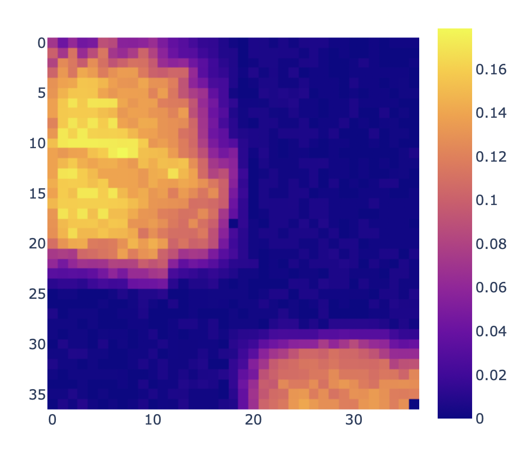
As compared to Experiment I, we can also see the agent exploring more and repeatedly visiting more states, which is the expected behavior as the optimal state is moving around.
Conclusion
If we were deploying a new solar panel anywhere in the world for some community with variable lighting, shading, potential panel issues, etc. we could say:
Place your panel anywhere you’d like facing any direction
Within a month or so, your panel will be producing about 90% of the optimal energy it could be
After about a year, your panel will be producing about 97% of the optimal energy it could be
After that, as the seasons change, shading changes, motors degrade, panel degrades, etc., your panel will learn on its own how to continuously optimize energy production without any external inputs or deterministic logic/controls/modeling required.
This was the exact objective of this project, and I’m incredibly excited that we’re seeing desired agent behavior now after numerous agent iterations, problem re-framings, and experiments.
You can see the final research summary below:


